Visualizing the 2019 Kincade Fire
The Python notebook and data file are available in this Github repository.
I recently developed an interest in using Python to analyze satellite imagery and geospatial data (in environmental and earth science contexts). So, I’ve been going through a number of different workshops and tutorials that are publicly available on Github. One of them is a workshop from the 2019 American Geophysical Union (AGU) conference titled “Snakes on a Satellite: Using Python and modern tools for research and analysis of next generation satellite data products”. In the tutorial, the authors go over a way to use a netCDF data file from the Suomi-NPP satellite to analyze aerosol optical depth (AOD) during the 2018 California wildfires.
While going through the workshop’s tutorials, I had some confusion about where to obtain a netCDF file such as the one used in the tutorial. Plus, given how wildfires were a big problem in 2019 as well for California, I was curious to apply the same methodology onto data from a 2019 wildfire. Thus, I decided to focus on the Kincade Fire, which spanned from late October 23, 2019 to November 20, 2019.
Analyzing data
Obtaining netCDF data on aerosol optical depth from NOAA
Observations on AOD can be obtained from the National Oceanic and Atmospheric Administration (NOAA)’s Comprehensive Large Array-data Stewardship System (CLASS). While trying to find out how to get my own NetCDF data, I found this link (clicking the link will start a PowerPoint file download) to a tutorial on how to order data from the CLASS website. That was useful in learning how to use the CLASS website; however, after going through the instructions and ordering my files through the website, I did not end up receiving my actual download files. NOAA is currently in the process of updating their site, so that could be why. Because of that, I decided to just try and download the file through the CLASS FTP site instead.
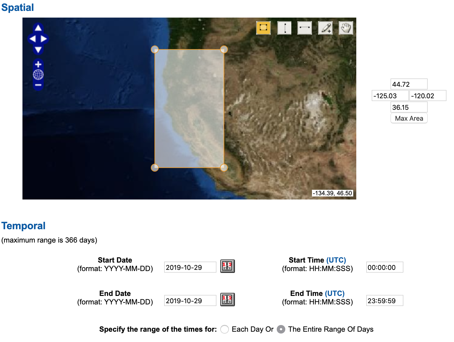
In order to figure out which netCDF file I want to download, I navigated to the CLASS home page. In the dropdown menu, I selected JPSS VIIRS Products (Granule) (JPSS_GRAN), then clicked GO. In the interactive map, under Spatial, I chose the general California geographic area. I decided to focus on just October 29, 2019 for this analysis.
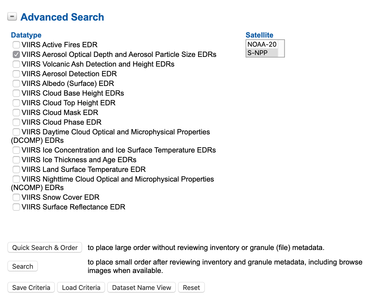
Then, under Advanced Search, I selected VIIRS Aerosol Optical Depth and Aerosol Particle Size EDRs as my Datatype and S-NPP as my Satellite. After that, I clicked on “Search” to see what results came up.
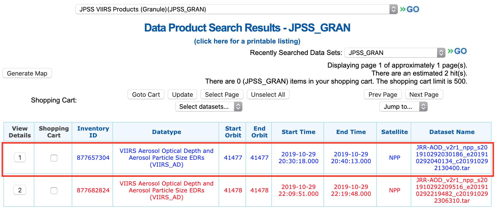
The results came up with two items to choose from. After clicking on Generate Map to see which I would prefer, I decided on the first item (the blue one), with the dataset name JRR-AOD_v2r1_npp_s201910292030186_e201910292040134_c201910292130400.tar.
So, next was a matter of figuring out how to navigate the FTP site and finding the exact file. The FTP site is organized by date, so I tried to find the data file I wanted as such: 20191029 ![]()
JPSS-GRAN ![]()
VIIRS-Aerosol-Optical-Depth-and-Aerosol-Particle-Size-EDRs ![]()
NPP. Or, click here to go straight to the right directory.
Upon arriving on the directory, I saw that none of the files matched the data file I wanted to download. Turns out, each of the .tar files in the directory included more .tar files, one of which is the one I wanted to download. Each .tar.manifest.xml file lists the files that are included in each corresponding .tar file. Instead of manually downloading each .tar.manifest.xml file and searching through each to find the data file I want, I needed to find a better way to find the right .tar file to download. So, what I did instead was utilize a few shell commands in Terminal to get the job down a lot quicker.
- I first downloaded all .tar.manifest.xml files in the directory using
wget:wget -r -nd -nH -A "*.tar.manifest.xml" ftp://ftp-npp.bou.class.noaa.gov/20191029/JPSS-GRAN/VIIRS-Aerosol-Optical-Depth-and-Aerosol-Particle-Size-EDRs/NPP/ - In each .tar.manifest.xml file, the names of the files included in the corresponding .tar file are kept within
<FileName>and</FileName>holders. Recall the file I wanted to download wasJRR-AOD_v2r1_npp_s201910292030186_e201910292040134_c201910292130400.tar. So, I used the followinggrepcommand to search through all .tar.manifest.xml files I downloaded to find the right file:grep -l '<FileName>JRR-AOD_v2r1_npp_s201910292030186_e201910292040134_c201910292130400.tar</FileName>' *The output of running that
grepline was:JPSS-GRAN_VIIRS-Aerosol-Optical-Depth-and-Aerosol-Particle-Size-EDRs_20191029_52685.tar.manifest.xml. That meant theJPSS-GRAN_VIIRS-Aerosol-Optical-Depth-and-Aerosol-Particle-Size-EDRs_20191029_52685.tarfile in the FTP directory holds the .tar file I wanted to download. - Finally, I used
wgetagain, this time to download the .tar file:wget -nd -nH ftp://ftp-npp.bou.class.noaa.gov/20191029/JPSS-GRAN/VIIRS-Aerosol-Optical-Depth-and-Aerosol-Particle-Size-EDRs/NPP/JPSS-GRAN_VIIRS-Aerosol-Optical-Depth-and-Aerosol-Particle-Size-EDRs_20191029_52685.tar
After the JPSS-GRAN_VIIRS-Aerosol-Optical-Depth-and-Aerosol-Particle-Size-EDRs_20191029_52685.tar file was downloaded and extracted, I saw the correct data file I wanted was there (except in .tar.gz format instead of just .tar). After extracting the JRR-AOD_v2r1_npp_s201910292030186_e201910292040134_c201910292130400.tar.gz file, I saw that there were multiple NetCDF files (.nc). I ended up quickly looking through each one in Python (using xarray) to see which areas each .nc file plotted, and I decided the JRR-AOD_v2r1_npp_s201910292033094_e201910292034336_c201910292124400.nc file was the most suitable one. So, that was the one I decided on to analyze and plot (it’s already included in the data folder in the Github repo).
Reading in netCDF data into Python
I used the xarray package, which is tailored for handling netCDF files. The information needed for plotting are the coordinates (Longitude and Latitude) and the data variable AOD550 (representing aerosol optical depths derived at 550 nm).
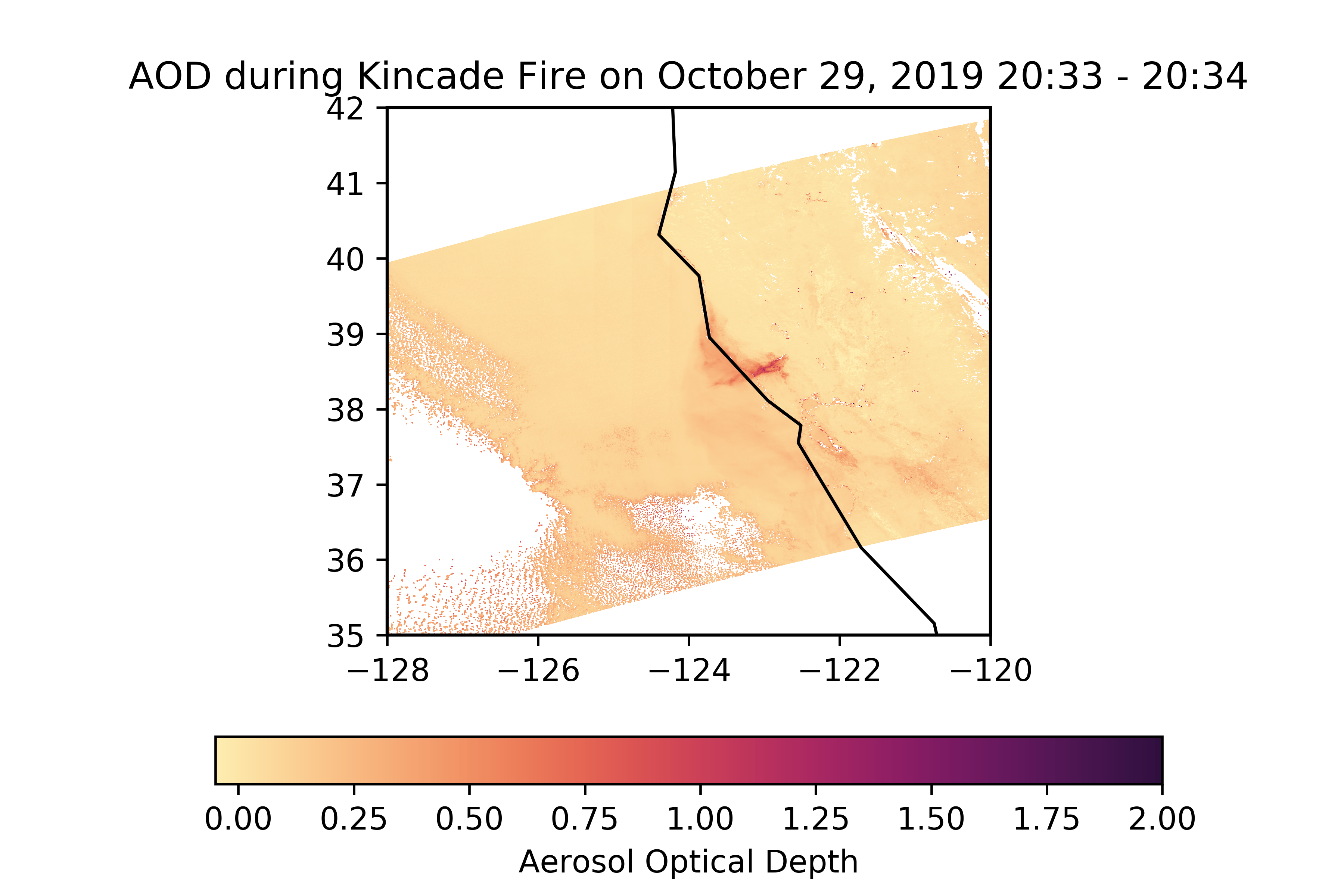
Plotting the aerosol optical depth
I used the matplotlib package to create the contour/mesh plot, as well as the cartopy package to change the projection of the map. The cmocean package has color palettes intended for making oceanography/water-related plots, but I liked the matter color palette, so I decided to use that for my contour color scale.